Partial Least Squares (PLS)
Lead Author(s): Danh Nguyen, PhD
Partial least squares can be viewed as a dimension reduction method that reduces the dimension of the predictor space by constructing a sequence of linear combinations of the original predictor variables. If we denote the predictors as X1, X2, . . ., Xp, then PLS dimension reduction reduces the p-dimensional predictor space into a lower K-dimensional component space. Depending on the area of application, the constructed linear combinations are called components, factors or latent variables. The PLS components are constructed by maximizing the sample covariance between the response vector y and linear combination Xc, where X is the n -by- p predictor matrix for n observations and vector c. So each PLS components is a linear combination
T = w1X1 + w2X2 + . . . + w p X p
and each component is orthogonal to every other component.
Examples and Implementation in SAS and R
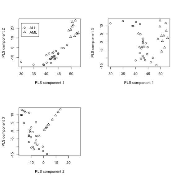
Example: Microarray gene expression data. Expression intensity measures for thousands of gene probes are simultaneously measured using microarrays, such as the Affymetrix array. In Golub et al. (1999)[ LINK to reference ]thousands of gene expressions are measured on a (training) data set of 38 samples, consisting of 27 acute lymphoblastic leukemia (ALL) samples and 11 acute myeloid leukemia (AML=1) samples. For illustration, a subset data set of p = 3051 gene probes is used here. An example of implementation using the R function PLS.r follows. >library(multtest) # to get Golub et al. (1999) leukemia data
>data(golub)
>X <- t(golub); dim(X) #[1] 38 3051
>y <- matrix(golub.cl) # sample labels: 27 ALL (0) and 11 AML (1)
>pls.fit <- PLS(X, X, y, 3) # fit PLS
The above PLS fit constructs 3 PLS components. The objects returned from fitting PLS are: > names(pls.fit)
[1] "W" "PVEX" "PVEY" "T1" "T2" "B" "V"
T1 consists of the three PLS fitted components. The PLS header function describes in detail the function inputs and outputs. Below are plots of the PLS components with markers for each type of samples (ALL or AML):
 The above PLS function provides the same results as the SAS implementation in PROC PLS[LINK to SAS reference]. Attached is a SAS macro for running a sample PLS: samplepls.txt.
PLS regression can also be implemented in R (pls [LINK - http://cran.r-project.org/] [LINK to section on PLS regression below.]
Other examples. PLS is often used in the field of chemometrics, with spectrometric calibration as a classic example. Here, spectrographic readings are taken at p frequencies or wavelengths on n samples of known concentrations. In clinical epidemiology, PLS dimension reduction has been applied to clinical variables such as dietary/nutrient intakes. Additional details can be found in the guide to SAS PROC PLS.
The above PLS function provides the same results as the SAS implementation in PROC PLS[LINK to SAS reference]. Attached is a SAS macro for running a sample PLS: samplepls.txt.
PLS regression can also be implemented in R (pls [LINK - http://cran.r-project.org/] [LINK to section on PLS regression below.]
Other examples. PLS is often used in the field of chemometrics, with spectrometric calibration as a classic example. Here, spectrographic readings are taken at p frequencies or wavelengths on n samples of known concentrations. In clinical epidemiology, PLS dimension reduction has been applied to clinical variables such as dietary/nutrient intakes. Additional details can be found in the guide to SAS PROC PLS.
Relation to Principal Components Analysis
Like PLS, Principal Components Analysis (PCA) also constructs orthogonal linear combinations of the predictors, but the linear combinations are constructed to maximize the variance of the linear combination of the predictors.
PCA Implementation in SAS and R. A standard R function to implement PCA is princomp when n > p. For cases where p > n, like genomics expression data, other functions can be used like eigen and svd. PCA can also be implemented in SAS using PROC PRINCOMP.
Partial Least Squares Regression (PLSR) and Principal Components Regression (PCR)
After fitting PLS, we have the K PLS components or linear combinations, say T1, T2, and TK. Partial least squares regression is a linear regression model [LINK to CTSpedia term or article on linear regression] with the K PLS components as predictors/covariates in the linear regression along with other relevant covariates, such as clinical and demographic variables. One can think of PLSR as a two-stage method. The first stage is the PLS dimension reduction. The second stage is the fitting of the linear regression. Here the outcome (response) variable Y is continuous.
In principal components regression, the above description is applicable with the PLS components replaced by the principal components in the regression model.
Partial Least Squares Classification
When the outcome variable is categorical and, for instance, the aim is to predict the diagnostic categories, then the interest is classification. For instance, in the examples section,[LINK back to above example/implementation section] one interest may be to explore the hypothesis of whether global gene expression profiles can predict correctly the acute leukemia subtypes (AML or ALL). Another example might include prediction/classification of controls and different stages of lung cancer based on biomarker data, such as gene expression (mRNA or protein) data obtained from microarray, or mass spectrometry etc.
Similar to PLSR, PLS classification involves using the constructed PLS components (possibly along with other clinical or demographic variables) in a classification procedure (second stage). There are many classification methods that can be used for this purpose, including linear or quadratic discriminant analysis, centroid methods, nearest neighbors, neural networks, etc. The book by Hastie et al. (2001)[LINK http://www-stat.stanford.edu/~tibs/ElemStatLearn/] may be useful to learn more about classification methods. See Nguyen and Rocke (2002)[LINK to reference] for examples of PLS cancer classification with genomic expression data.
Implementation Considerations
There are considerations when performing PLS regression or classification:
- Standardization: In the PLS dimension reduction step, centering and/or scaling may be needed.
- Generalization and over-fitting: With sufficient data, a training (learning) data set and a test data set should be created to test how well the fitted model performs on new (test) data. For instance, the original data can be divided into 2/3 and 1/3 for training and testing. If this is not feasible, cross-validation (one one out or M-fold CV) is an alternative.
- In fitting the PLS using the PLS.r [LINK] function with training and test data:
>pls.fit <- PLS(X.train, X.test, y, 3) # fit 3-component PLS
the outputs T1 and T2 are the training and test components respectively. The PLS() function also can take more than one outcome variables (continuous or G categories/groups), in which case Y is a matrix. When there are G groups for a categorical outcome, then Y is a matrix of indicator variables. See PLS( ) function header for more details.
See Also
References
- Danh V. Nguyen: UC Davis \x{2013} CTSpedia article and R functions. (February 14, 2009)
- Golubetal.(1999).Molecularclassificationofcancer:classdiscoveryandclasspredictionbygeneexpressionmonitoring,Science,Vol.286:531-537.http://www-genome.wi.mit.edu/MPR
- Hastie, T., Tibshirani, R., Friedman, J. (2001) The Elements of Statistical Learning: Data Mining, Inference, and Prediction. Springer, New York.
- Nguyen Rocke (2002)Tumor classification by partial least squares using microarray gene expression data. Bioinformatics, 18, 39-50.
- SAS PROC PLS. SAS User\x{2019}s Guide. Cary, N.C.

