Note: Start and end dates are relative to day "0," durations are in days. However, the other 20 of the 50 patients are unaccounted for since Dr. Taylor was doing a prevalence study and did not want to collect retroactive data. The following is a plot of the longitudinal lines of each of the 50 patients: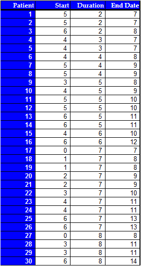
NOTE: Blue lines represent sampled patients, black lines represent unsampled patients with symptoms. The red line represents the time of the cross-section. Dr. Taylor calculates the mean of the sampled durations to be 5.6 days, and wants to conclude that the mean duration of flu symptoms in her patients is higher than the average duration that the CDC predicts (suppose arbitrarily that the predicted range for the particular year is 2-5 days). However, to do so would be a mistake because there is a bias in the data collected. Return to Top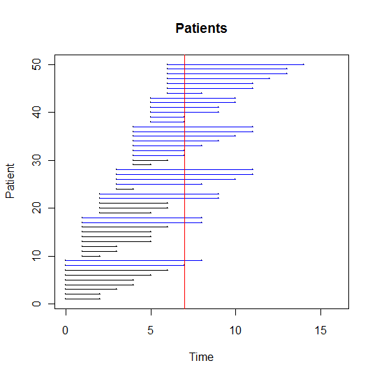
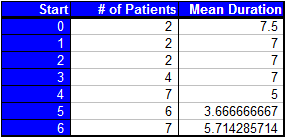
The first indicator of length bias is that, on average, the number of patients in the categories of later start dates are higher than those in the categories of earlier start dates. The problem with this is that we suspect that the start dates of patients should be relatively uniform throughout the 7 days. This means we are probably sampling only the longer durations from the categories with earlier start dates. Also, as we suspected, the mean durations per category seem to be higher (on average) for those sampled that started having symptoms closer to day zero. We could verify this by way of linear regression if it were not clear and look for a decreasing trend in the plot of start date versus mean duration. In fact, for this case the slope of the regression line is -0.5009. Our conclusion is that there is some length bias in our sampling procedure. Return to Top
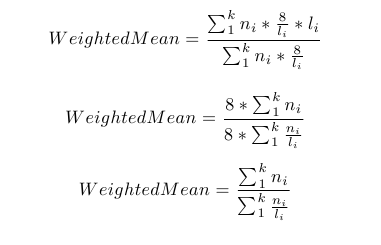
The next step is to come up with the weights on our measurements. In our case, it is convenient to weight our measurements in term of the largest measurement (8 days). For example, we are eight times as likely to observe a measurement of length "8" over a measurement of length "1." Thus, we weight the number of measurements of length 1 day (in our case, none) by a factor of 8. The generalized form of our weights in this study is weight = 8/duration. So in order to find our corrected mean we use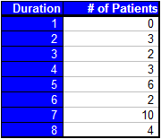
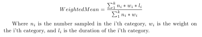 The idea behind this corrected mean is that it up-weights the number of short observations and therefore the total duration per category. Another way to think of it is that in our weighted mean calculation we are increasing the proportion of shorter observations. We then divide by the weighted number of observations to calculate the weighted average duration per patient. In this particular case, since our weights are based on the length of the durations, our formula happens to simplify to
 It is conceivable that this simplified formula may not always work, depending on what we choose as our weights.
Now it is time to compare the uncorrected mean, the corrected mean, and the true mean durations of the patients' flu symptoms in Dr. Taylor's sample (the data used to calculate these quantities, and a program to calculate them can be found attached).
The uncorrected mean was already noted to be 5.6 days, the corrected mean turns out to be 4.62 days, and the true mean (which we know since this study is a simulation and we have access to the data from all of the patients not in the sample) is 4.70 days. Thus, our corrected mean is much closer to the true mean of the population and we have a mean duration of flu symptoms in Dr. Taylor's practice which is within the CDC's predicted range.
It is conceivable that this simplified formula may not always work, depending on what we choose as our weights.
Now it is time to compare the uncorrected mean, the corrected mean, and the true mean durations of the patients' flu symptoms in Dr. Taylor's sample (the data used to calculate these quantities, and a program to calculate them can be found attached).
The uncorrected mean was already noted to be 5.6 days, the corrected mean turns out to be 4.62 days, and the true mean (which we know since this study is a simulation and we have access to the data from all of the patients not in the sample) is 4.70 days. Thus, our corrected mean is much closer to the true mean of the population and we have a mean duration of flu symptoms in Dr. Taylor's practice which is within the CDC's predicted range.
| I | Attachment | Action | Size | Date | Who | Comment |
|---|---|---|---|---|---|---|
| |
|
manage | 1 K | 21 Jul 2010 - 20:05 | UnknownUser | Data from all 50 patients |
| |
|
manage | 3 K | 21 Jul 2010 - 17:03 | UnknownUser | Categories based on start dates |
| |
|
manage | 2 K | 21 Jul 2010 - 17:24 | UnknownUser | Categories based on durations |
| |
|
manage | 11 K | 21 Jul 2010 - 15:34 | UnknownUser | Longitudinal lines chart |
| |
|
manage | 11 K | 21 Jul 2010 - 15:51 | UnknownUser | |
| |
|
manage | 13 K | 20 Jul 2010 - 21:59 | UnknownUser | Data from all sampled patients (30) |
| |
|
manage | 2 K | 21 Jul 2010 - 20:02 | UnknownUser | Simulation Program for data and analysis |

